Overview

Teaching: 10 min
Exercises: 10 min

Questions

• How does one train machine learning models in python?

Objectives

• Train a Random Forest model.

• Train a neural network model.

Models

In this section we will examine 2 different machine learning models \(f\) for classification: the random forest (RF) and the fully connected neural network (NN).

Random Forest

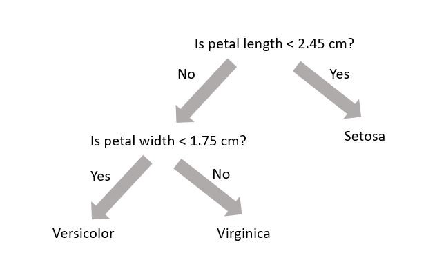
A random forest (see Chapter 7) uses decision trees (see Chapter 6) to make predictions. Decision trees are very simple models that make classification predictions by performing selections on regions in the dataset. The diagram below shows a decision tree for classifying three different types of iris flower species.

A decision tree is not trained using gradient descent and a loss function; training is completed using the Classification and Regression Tree (CART) algorithm. While each decision tree is a simple algorithm, a random forest uses ensemble learning with many decision trees to make better predictions. A random forest is considered a black-box model while a decision tree is considered a white-box model.

Model Interpretation: White Box vs. Black Box

Decision trees are intuitive, and their decisions are easy to interpret. Such models are considered white-box models. In constrast, random forests or neural networks are generally considered black-box models. They make great predictions but it is usually hard to explain in simple terms why the predictions were made. For example, if a neural network says that a particular person appears on a picture, it is hard to know what contributed to that prediction. Was it their mouth? Their nose? Their shoes? Or even the couch they were sitting on? Conversely, decision trees provide nice, simple classification rules that can be applied manually if need be.

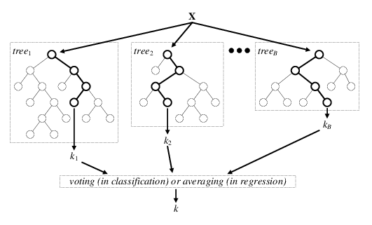
The diagram below is a visual representation of random forests; there are \(B\) decision trees and each decision tree \(\text{tree}_j\) makes the prediction that a particular data point \(x\) belongs to the class \(k_j\). Each decision tree has a varying level of confidence in their prediction. Then, using weighted voting, all the predictions \(k_1,...k_B\) are considered together to generate a single prediction that the data point \(x\) belongs to class \(k\).

Wisdom of the Crowd (Ensemble Learning)

Suppose you pose a complex question to thousands of random people, then aggregrate their answers. In many cases you will find that this aggregreated answer is better than an expert’s answer. This phenomenon is known as wisdom of the crowd. Similarily, if you aggregrate the predictions from a group of predictors (such as classifiers or reggressors), you will often get better predictions than with the individual predictor. A group of predictors is called an ensemble. For an interesting example of this phenomenon in estimating the weight of an ox, see this national geographic article.

In the previous page we created a training and test dataset. Lets use these datasets to train a random forest.

from sklearn.ensemble import RandomForestClassifier

RF_clf = RandomForestClassifier(criterion='gini', max_depth=8, n_estimators=30)
RF_clf.fit(X_train, y_train)
y_pred_RF = RF_clf.predict(X_test)

# See how well the classifier does
print(accuracy_score(y_test, y_pred_RF))

1. The classifier is created. In this situation we have three hyperparameters specified: criterion, max_depth (max number of consecutive cuts an individual tree can make), and n_estimators (number of decision trees used). These are not altered during training (i.e. they are not included in \(\theta\)).
2. The classifier is trained using the training dataset X_train and corresponding labels y_train.
3. The classifier makes predictions on the test dataset X_test. The machine learning algorithm was not exposed to this data during training.
4. An accuracy score between the test dataset y_test and machine learning predictions y_pred is made. The accuracy score is defined as the ratio of correctly identified data points to all data points.

Neural Network

A neural network is a black-box model with many hyperparameters. We will discuss the mathematical structure of neural networks later on in the tutorial. If you are interested in neural networks, I would highly recommend reading Chapter 10 of the text (and Chapters 11-18 as well, for that matter). It is also discussed here in the tutorial. To use a neural network with sci-kit learn, we must modularize its construction using a function. We will later pass this function into a keras wrapper.

def build_model(n_hidden=1, n_neurons=5, learning_rate=1e-3):
    # Build
    model = keras.models.Sequential()
    for layer in range(n_hidden):
        model.add(keras.layers.Dense(n_neurons, activation="relu"))
    model.add(keras.layers.Dense(2, activation='softmax'))
    # Compile
    optimizer = keras.optimizers.SGD(lr=learning_rate)
    model.compile(loss='sparse_categorical_crossentropy', optimizer=optimizer, metrics=['accuracy'])
    return model

For now, ignore all the complicated hyperparameters, but note that the loss used is sparse_categorical_crossentropy; the neural network uses gradient descent to optimize its parameters (in this case these parameters are neuron weights). The network can be trained as follows:

X_valid, X_train_nn = X_train[:100], X_train[100:]
y_valid, y_train_nn = y_train[:100], y_train[100:]

NN_clf = keras.wrappers.scikit_learn.KerasClassifier(build_model)
NN_clf.fit(X_train, y_train, validation_data=(X_valid, y_valid))
y_pred_NN = NN_clf.predict(X_test)

# See how well the classifier does
print(accuracy_score(y_test, y_pred_NN))

The neural network should also have a similar accuracy score to the random forest. Note that while the accuracy is one metric for the strength of a classifier, many other metrics exist as well. We will examine these metrics in the next section.

Accuracy: The Naive Metric

Suppose you have a dataset where 90% of the dataset is background and 10% of the dataset is signal. Now suppose we have a dumb classifier that classifies every data point as background. In this example, the classifier will have 90% accuracy! This demonstrates why accuracy is generally not the preferred performance measure for classifiers, especially when you are dealing with skewed datasets. Skewed datasets show up all the time in particle physics where one has access to many more background than signal events. In this particular tutorial, we have a dataset with 520000 background events and 370000 signal events.

Key Points

• Random Forests and neural networks are two viable machine learning models.